Mantle Convection
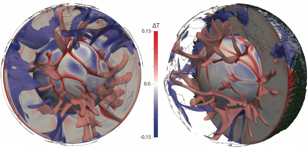
From simple box models to global spherical simulations like the one above - learn to simulate mantle convection step by step.
The diagram below shows the suite of G-ADOPT notebook tutorials for mantle convection, and how they build on one another. Together, these tutorials demonstrate how to set up and run both forward and inverse mantle dynamics simulations using G-ADOPT.
graph TD
  base[Base]

  subgraph model_diagnostics[Model Diagnostics]
  dynamic_topography[Dynamic Topography]
  end

  subgraph adjoint[Adjoint]
  adjoint_forward[Forward] --> inverse[Inverse]
  end

  subgraph geometry[Geometry]
  cylindrical_2d[2D Cylindrical] --> spherical_3d[3D Spherical]
  end

  subgraph gplates[GPlates]
  gplates_global["Global GPlates"]
  end

  subgraph dimension[Dimension]
  cartesian_3d[3D Cartesian]
  end

  subgraph bcs[Boundary Conditions]
  free_surface[Free Surface]
  end

  subgraph compressibility[Compressibility]
  tala[TALA] --> ala[ALA] --> visualise_ala[ALA Nullspace]
  end

  subgraph rheology[Rheology]
  viscoplastic[Viscoplastic] --> drucker_prager[Drucker-Prager]
  end

  base --> dimension
  base --> compressibility
  base --> rheology
  base --> geometry
  base --> bcs
  base --> adjoint
  base --> model_diagnostics
  geometry --> gplates

  click base "base_case"
  click tala "2d_compressible_TALA"
  click ala "2d_compressible_ALA"
  click visualise_ala "visualise_ALA_p_nullspace"
  click viscoplastic "viscoplastic_case"
  click drucker_prager "Drucker_Prager"
  click cartesian_3d "3d_cartesian"
  click cylindrical_2d "2d_cylindrical"
  click spherical_3d "3d_spherical"
  click gplates_global "gplates_global"
  click adjoint_forward "adjoint_forward"
  click inverse "adjoint"
  click free_surface "free_surface"
  click dynamic_topography "dynamic_topography"
Our tutorials take you on a journey from the simplest model setups to advanced, Earth-like simulations. Starting with a basic 2D convection model (isoviscous, incompressible), you will gradually explore more realistic physics, new boundary conditions, 3D and spherical geometries, and even link your models to plate reconstructions with GPlates.
Along the way, you will also discover how to analyse key surface signals such as dynamic topography and learn how to use G-ADOPT's powerful adjoint tools to recover unknown conditions from data.
After completing these tutorials, you will be equipped to:
- Build forward mantle convection models from simple boxes to full spherical shells.
- Incorporate realistic physics such as visco-plastic rheology and compressibility.
- Apply boundary conditions including free surfaces and reconstructed plate motions.
- Compute and interpret dynamic topography.
- Use adjoint methods to invert for unknown initial conditions.
Whether you are new to mantle dynamics or ready to tackle state-of-the-art research problems, these tutorials provide a clear step-by-step path into mantle convection modelling with G-ADOPT.